SUMMARY
Utilities are unnecessarily limited by their ability to explore and quickly test hypotheses about data and then to move analytic use cases from prototypes to production in operational systems. This arises because utilities are very slow to traverse the analytics pipeline. The analytics pipeline not only supports the implementation of applications for previously identified use cases, but also enables the discovery of new use cases through exploration of the available measurement data. The reasons for utilities’ sluggishness in traversing the pipeline were highlighted extensively in last year’s Learning from Data Grid of the Future paper [1]. Fundamentally, utilities are tied to legacy platforms, ill equipped for analytics, and need the right tools to process and analyze time series sensor data at scale.
In this paper, we present an alternative vision by demonstrating the rapid development and deployment of an analytic use case enabled by a universal sensor analytics platform. Voltage sag detection was chosen as the example use case as it is useful to utilities, visually compelling, and highlights many of the important features of the analytics platform. Crucially, while the voltage sag detection described in this paper is not novel in itself, it was completed, from prototype to production, in approximately one work week. This is dramatically less time than is currently possible in the industry. Such short development times afford utilities numerous benefits including the ability to develop and deploy many novel analytics, to test multiple approaches for accomplishing certain analytic goals, to conduct sandbox testing without committing enormous amounts of time, and even to tailor analytics to the requests of operators in real time.
KEYWORDS
real time analytics, time series, sensor data, big data, analytic use cases, production data platform
1.INTRODUCTION
1.1The Problem
Surveying the utility landscape, we see an ever-present chasm in the grid analytics space. This gap prevents utility engineers’ and researchers’ ideas and hypotheses about how data from PMUs and other sensors can create value from being fully developed as prototype use cases and then deployed into production. Currently, at best, these ideas get implemented in MATLAB and run on a laptop, with results potentially presented at conferences or published in journals. However, even successful prototypes that enhance the grid’s stability, resiliency, and/or reliability can take years to be operationally deployed if they even make it to the production environment.
The development of oscillation detection, a wide area monitoring use case for synchrophasors, is a great example of this problem. In 2003, PSERC developed a project on real-time oscillation monitoring. In a 2008 report to NASPI [2], the project team reported that a prototype of the algorithm had been installed at Entergy and TVA in 2006. It took nearly three years to get to a prototype implementation and another two years to deploy the prototype into a production PDC for a total of five years from prototype to production.
The slow pace of analytic use case development has allowed high-value data to languish unused at utilities and even to be deleted due to storage space and dated software cost models. This limited use of sensor data inhibits the utility’s ability to push the boundaries of their technical capabilities and gain greater insight into the real-time operation of their networks. As phasor measurement capabilities are built into many smart assets such as modern smart relays, the number of PMUs connected to the grid is already in the hundreds of thousands [3]. Many transmission utilities have dozens, hundreds, or even thousands of PMUs deployed but inactive, lacking the capabilities to leverage the vast data volumes that these sensors generate when operational.
By keeping the PMU capabilities disabled, utilities forsake a massive load of geographically extensive, time synchronized, high resolution information about their networks. Many applications of sensor data become increasingly accurate with increased network coverage and some are only feasible when measurement coverage exceeds a minimum threshold. Therefore, artificially restricting the number of sensor data streams used because of legacy platform limitations not only discards measurements from certain sensors, but also reduces the value and power of the measurements that are collected.
The high investment of time required to deploy new analytics means that utilities cannot quickly compare several approaches to a particular use case to determine which performs best. This widens the chasm further, especially for analytic use cases where a vast number of new techniques, tested in simulation alone, are proposed each year, such as fault identification and localization [4, 5, 6]. Rather than being an asset, the vast literature of algorithmic options is a daunting prospect, since comparing several techniques is essentially infeasible, and selecting any one seems risky.
1.2Analytics Pipeline Review
The analytics pipeline (Figure 1) is a general sequence of steps to realize value from data that applies to the development of analytic use cases not just in utilities but also in many other data intensive industries and research areas including finance, healthcare, medical imaging and diagnostics [7], astronomy, and the broader energy sector.
Notice that the “Analysis and Modeling Stage,” focusing on the development and refinement of the use case, is highly iterative in nature. This is not to say that no other feedback loops exist within this process but rather that this one is especially important for use case development.
The 2017 Grid of the Future paper, Learning from Data: Fixing the Analytics Pipeline to Increase the Rate of Grid Evolution, detailed both how and why each stage of this process is unnecessarily hampered by numerous factors. Ideas and hypotheses about how data could be useful are realized via the traversal of the analytics pipeline with the last stage seeing the ideas operationalized inside the utility. Potential new use cases fall short of production deployments in two general ways.
- Some use cases never get fully realized because traversing stages 0 through 5, from data capture to visualization, reporting and propagation of analytic results, is both time and resource intensive for numerous reasons, detailed previously [1].
- The use cases that successfully refined to a production-ready state still face a chasm transitioning from prototypes into production for everyday use within utilities.
This paper demonstrates that it is possible to develop and deploy an analytic for grid sensor data in days rather than months or years by walking through the steps taken to achieve these results. The key to such speed is the use of an open, state-of-the-art platform to ingest, store, clean, visualize, and process data from such grid sensors such as PMUs, digital fault recorders, point on wave sensors, smart meters, and power quality meters. This universal sensor analytics platform was designed with a deep understanding of the analytics pipeline to allow utilities and other organizations to traverse it at warp speed. The platform allows authorized utility users to easily access data and enables artificial intelligence and analytics as core components of the platform (instead of bolted on additions), making available best of breed open source data visualization, analysis, and machine learning software libraries. The paper, A Universal Platform for Utility Sensor Data Analytics and Artificial Intelligence, details this universal sensor analytics platform, describing the underlying technologies and innovations that enable such capabilities [8].
1.3Example Analytic: Identification of Voltage Sags
Detecting voltage sags is a very specific type of univariate event detection of interest to both transmission and distribution utilities. In a voltage sag, the voltage temporarily decreases and then returns to the approximately original value over a specified, brief period of time. The causes of voltage sags in both transmission and distribution networks are varied and include switching operations, faults, and inrush currents. Voltage sags can cause sensitive loads, especially those of industrial customers, to drop offline [9, 10]. Quantifying the number and size of voltage sags in historical data is therefore a useful method to assess the health of utility systems. An excessive number of voltage sags can indicate underlying issues in equipment or control processes and may necessitate corrective actions.
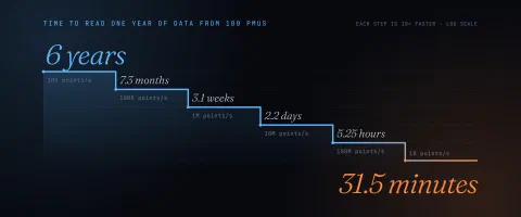
We develop an analytic to detect transient decreases in voltage magnitude measurements from synchrophasor sensors. To detect the voltage decreases, we want to scan every voltage phasor magnitude measurement and identify each voltage sag, the timestamp when occurred, and quantify its percentage size. Synchrophasor data is perfect for this application because its intrinsically high sample rate--30 Hz or greater--allows observation of short-duration, sub-second events that span only a few cycles. However, scanning a year of just a single voltage phasor magnitude signal at 120 Hz requires the processing of 3,784,320,000 data points or approximately 60GB of time series data.
The development of such an analytic follows a sequential yet iterative process, starting with exploration and ending with an analytic ready for production. Ideally, the engineer or analyst first explores the operational data visually to get a better “sense” or “feel” of the data, randomly sampling voltage phasor magnitudes, searching for voltage sags to collect examples of the phenomenon to develop initial concepts for the detector. The next step is the development of different approaches to identifying such events and then test each on subsets data. With a promising approach identified, larger scale testing is required. Key to this step is the visualization of the algorithm’s performance so that the effectiveness of the prototype can be determined and then demonstrated to an audience. Finally, if requirements have been met the approach can be deployed to production to become available to all users of the system or the prototype algorithms can be refined and re-tested.
2.ANALYTICS AT WARP SPEED
To accelerate analytics, the early stages of the analytics pipeline are handled by the universal sensor analytics platform and require little additional effort on the part of the user. The data capture of stage 0 can be verified simply through the rapid visualization of the data in the multi-resolution plotter. Stages 1 and 2—access and acquisition—are also handled by the database and its API. The database allows data to be either manually downloaded using the plotter interface or to be programmatically queried via the API, both orders of magnitude faster than legacy historians. In addition, the density of available data points per data stream can be viewed in the top segment of the plot (see top of Figure 2). This visualization partly addresses stage 3 of the analytics pipeline: data wrangling and cleaning. Using the density information, it is possible to easily identify a time span over which the data of interest is available without missing or repeated values--both of which are common problems when working with grid sensor data.
2.1Data Exploration
Analytic development often begins with data exploration, a step whose value is difficult to overemphasize, especially when the user is unfamiliar with the measurement data or the phenomenon of interest. Pervasive sensor data, especially continuous, high frequency measurements of the electric grid, is relatively new, and some sensors, such as distribution synchrophasors (µPMUs), are novel. Many utilities and academic researchers are unfamiliar with the sensor measurements or only have experience with simulated versions different from real data. For example, there is some uncertainty about the meaning of µPMU measurements [11]. During transient events such as faults or when the system frequency is not constant, the voltage and current do not follow the perfect sinusoidal model--with a 60Hz frequency and fixed amplitude and phase. However, the PMU always outputs a magnitude and angle measurement that implicitly assumes this perfect model. Therefore, the physical interpretation of the returned magnitude and angle measurements can be ambiguous. Voltage sags have a very distinctive appearance in PMU voltage magnitude measurements. However, users familiar with point-on-wave or lower resolution measurements may not immediately recognize the right metric to isolate these events in PMU magnitude data. Therefore, exploring the data and gaining familiarity with these novel data sets is a vital first step in developing new applications.
The universal sensor analytics platform enables exploration of high volume, high resolution, multi-modal grid sensor data via rapid data access and interactive, multi-stream visualization across time scales [12]. Given this capability, voltage sags can be identified at the lowest temporal resolution, where months or years of data are visible (top panel, Figure 2). The visualization not only shows the average value for the time period represented by a single pixel column but also shows the minimum and maximum values as a shaded region. Thus, even at this resolution, voltage decreases are visible as fine spikes. Traversing the panels in the Figure 2 from top to bottom, each shows an increased level of “zoom” or finer temporal resolution and required a separate query of the platform. Each query completed in less than 200 milliseconds making truly interactive data exploration possible [13]. With the platform, the user can select an area of interest, shown in red, and smoothly zoom in to resolve individual 120Hz measurements. At this level of zoom, the exact shape of the transient voltage decrease is evident. After examining numerous such events, the user is armed with intuition for what makes these events unique and can start to prototype a potential detection approach.
2.2Rapid Prototyping
To quickly prototype this idea, Jupyter Notebook and the Python API are used. Jupyter Notebooks contain both computer code (e.g. python, R, MATLAB, or other languages) and rich text elements such as text paragraphs, equations, figures, URL hyperlinks, and even dynamic, interactive visualizations. Therefore, notebooks are human-readable and executable including both the scripts used to perform data analysis as well as the results (figures, tables, etc.) and documentation text [14].
The general approach to voltage sag detection is to compute a metric on a window of data that indicates the presence of a voltage sag. Based on the data exploration step, the voltage sag’s shape suggests several potential metrics. The first possibility, Voltage Sag Metric 1 or VSM-1, finds the minimum value within the signal segment and computes the differences between this minimum value and the measurements shortly preceding and following it (both differences are expected to be large). The second possibility, VSM-2, calculates the difference between the window’s mean and minimum (expected to be large) and the difference between the window’s maximum and mean (expected to be small). Metric two ensures that the voltage sag consists of a narrow spike that drops significantly below an otherwise predominantly flat signal.
Using the Python API, test segments of data that include voltage drops as well as other notable changes that are not voltage drops found via data exploration are pulled into the Jupyter Notebook. Next, the two proposed voltage sag metrics are computed over the samples to get a sense of their efficacy. The implementation of the first metric in the notebook is shown in Figure 3. Each proposed metric consists of two values and can be quickly evaluated using a scatter plot Figure 4. This preliminary result suggests that both metrics are effective for detecting voltage sags.
After verifying the promise of the two approaches on a few samples, the speed of the platform enables testing over a much larger data set before being deployed to production. VSM-1 requires scanning through all of the data, querying the database for full resolution measurements (120Hz). Implementing this is as simple as putting our scripts from the exploratory phase into a for loop. Over one day of voltage magnitude measurements, the first approach runs in 23 minutes or 63x real time. The algorithm detected six suspected voltage sags.
Metric two can be similarly implemented by querying the data at full resolution within a for loop. However, the formulation of the metric allows us to leverage an important aspect of the platform to achieve even faster performance. In addition to raw values, the universal sensor platform stores summary statistics at the internal nodes of its tree structure. At a particular internal node, the summary statistics consist of the mean, minimum, and maximum over all values “below” that node. These summary statistics can be queried more rapidly than the raw values. Since metric two is defined only in terms of the mean, minimum, and maximum over a window, we can compute it by querying the summary statistics for the window. Over the same day of voltage magnitude measurements, the approach runs in 1.28 seconds or 67750x real time. This algorithm detected the same six suspected voltage sags as VSM-1.
In this test case, the two approaches have dramatically different runtimes but detect the same events. This may not always be the case and using summary statistics inherently limits the range of analytics possible compared to using the raw, full resolution data. However, as this example demonstrates, the power of the platform is that both approaches can be prototyped and tested rapidly so the appropriate tradeoffs between speed and accuracy can be chosen.
2.3Test and Evaluation
Visualization is an important sub-step of the Analysis and Modeling step, especially when using data consisting of multiple, high resolution streams, as is the case for PMU measurements. Furthermore, visualizations can be highly convincing communication tools, allowing the analyst to disseminate the analytic results to a wider audience. Jupyter notebooks with the Python kernel offer the user a plethora of open source visualization tools—including packages such as Matplotlib, Altair, and Seaborn—giving an extraordinary variety of ways to test, evaluate, and communicate results. This section demonstrates the potential to create compelling and even attractive visualizations for our voltage sag detection problem.
The performance of the voltage sag detection metric over a full day of data can be visualized with a scatter plot shown in Figure 5. While a few non-voltage sag events can come close, the simple constant thresholds used, indicated by blue dashed lines, seem appropriately set for detecting outliers. Also note that the voltage sag points lie close to the x=y line, indicating that the pre- and post-sag voltage levels are very close for this set of events.
Based on the visualization in Figure 6, the detected voltage sags are indeed real voltage sags with a distinctive and consistent shape, validating this metric for a larger sample of data. Additional analyses can be easily visualized to offer more insights into the voltage sags and the event detection approach. A heat map (Figure 7) indicates the sensor locations where voltage sags occur over a month and a histogram (Figure 8) demonstrates the size distribution of the sags. From the heatmap, we see that sensor 1 captures many voltage sags throughout the first part of the month. This may indicate the presence of a periodic load near that particular PMU which becomes inactive during the second part of the month.
From the histogram, we see that most of the detected sags during the month are small--well below the 10% level that would be noticed by the utility. Therefore, from the perspective of voltage sags, this feeder does not appear to have any serious issues for the month analyzed. Nevertheless, the visualizations are a quick and effective way to ascertain that the feeder has no issues and to determine potentially problematic points. For example, the presence of a periodic load near sensor 1, evident in the heat map visualization, suggest that this might be a good location for system operators to monitor and check on first when issues do arise.
2.4.Deploying Analytics to Production
The key difference between the prototype analysis and the move to production arises from the size of the data. During prototyping, a subsample of the data is interrogated locally on the analyst’s or engineer’s laptop. This requires the data to be transmitted from the production system, over the network, to the laptop. Due to the size of the data—one year of a single voltage magnitude phasor is over 30GB in size—and network bandwidth, prototype is often limited to testing subsets of the data and another mechanism is required to deploy the analytic to the full data set. Instead of moving the terabytes or petabytes of data to the calculation, successful big data platforms use data locality and move the algorithms and calculations to the data; source code describing the analytic is orders of magnitude smaller than the data.
The DISTIL framework used by the universal sensor analytics platform leverages this same approach. DISTIL was created to enable the rapid development of scalable analytics pipelines with strict guarantees on result integrity despite asynchronous changes in data [15]. DISTIL is composed of two separate components: (1) distillers that apply a function to each data point or window of data points in one or more time series and (2) the distil processing framework that handles the performance optimizations and bookkeeping associated with multiple interleaved streams arriving at different rates, possibly out of order, chunking, buffering, scheduling and so on. Distillers are the “user-facing” portion of DISTIL. At the heart of each distiller is a smaller kernel, that contains two functions; (1) the precompute allows the user to specify what data will be needed for the (2) compute function that will operate on the data and return the computed values and associated time ranges. This model of analytics covers a large number of potential operations and analytics that can be performed on time series data.
To implement the voltage sag detection analytic in distillate form, the analyses developed in the Jupyter notebook were translated into the Go Programming language. We chose to implement metric one as a distiller, as it scans every raw data point in the stream, as opposed to only summary statistics. Go is an open-source language in the C family developed by Google to make distributed, systems software engineering far easier for the developer [16]. Once the algorithm has been developed in the Jupyter environment, where its efficacy can be easily ascertained and evaluated through mathematical analysis and visualizations, the translation to Go is simple. However, some properties of the distil framework must be kept in mind when doing the translation, and occasionally the analytic algorithms must be adjusted to account for these. For example, distillers can be called on arbitrary length data segments in non-chronological order, so the processing code within a distiller must be structured to be stateless and idempotent. To guarantee a certain length of the data chunk is passed to the distiller for processing, the number of “leading points” must be set. These are points immediately preceding the block to be processed. The voltage sag detection method requires a window of data with length greater than or equal to the maximum duration of a voltage sag. We therefore specify a certain number of leading points when creating our distiller and then implement the algorithm in much the same form as in the Jupyter notebook.
Though it scans through every single measurement point, the distiller processed the entire dataset, approximately 200 days of data, in 125 minutes or 2300x real time. Apart from speed, there are other advantages to creating a distillate of the voltage sag analytic. The distillate stream only contains a point with value 1 at the time of a detected voltage sag and is, therefore, much lower density than the original data. It is easy to visualize the voltage sag locations by viewing the distillate stream in the Plotter (Figure 9). This visualization also leverages all the convenient multi-resolution features of the Plotter. Another analytic could quickly localize the voltage sags using the voltage sag distillate points, without processing all the original measurement points. This has great performance benefits. Finally, the distiller can be conveniently and quickly run on multiple or all data streams and will continue to detect voltage sags as new measurement data streams to the database.
3.CONCLUSION
Utilities are dramatically limited in their ability both to test hypotheses and use cases leveraging data and to move prototype analytics into full deployment in production systems. To show that the status quo is not some fundamental limitation, this paper demonstrates not only the rapid development of a use case of interest using high density PMU data but also the deployment of this use case to a production big data system with operational data. This rapid traversal of the analytics pipeline was made possible through the use of a third-generation big data system custom designed for utility sensor data.
This use case is also particularly effective for demonstrating the power of the advanced sensor analytics platform to enable analytics development and deployment at warp speed. By definition, voltage sags are brief events lasting for as short as half a cycle or up to one minute [9]. Therefore, in terms of the number of data points involved, detecting these events is akin to finding a needle in a haystack. For example, in order for a distribution synchrophasor reporting at 120Hz to detect a voltage sag over one day of measurements, the platform must process tens of millions of data points per stream to identify an event spanning on the order of tens of data points. Note that we are but scratching the surface of the tip of the iceberg with regards to event detection. This paper focused on identifying a particular, simple pattern within voltage phasor magnitude data stream that could be captured by simple statistical descriptors. There are numerous other event types and patterns to be discovered in PMU data that will lead to new for utilities.
BIBLIOGRAPHY
- [1] Murphy, SP and Jones, KD, “Learning from Data: Fixing the Analytics Pipeline to Increase the Rate of Grid Evolution,” 2017 Grid of the Future Symposium, Cleveland, OH, Oct, 2017.
- [2] Venkatasubramanian MV, and Carroll R, Oscillation Monitoring System, NASPI Meeting, Charlotte, October 2008
- [3] Schweitzer EO, Keynote Presentation, 2017 Reliability Leadership Summit, Washington, DC, March 21, 2017.
- [4] Yu, Chi-Shan, et al. “A new PMU-based fault location algorithm for series compensated lines.” IEEE Transactions on Power Delivery 17.1 (2002): 33-46.
- [5] Jiang, Joe-Air, et al. "An adaptive PMU based fault detection/location technique for transmission lines. I. Theory and algorithms." IEEE Transactions on Power Delivery 15.2 (2000): 486-493.
- [6] Lien, Kai-Ping, et al. "Transmission network fault location observability with minimal PMU placement." IEEE Transactions on Power Delivery 21.3 (2006): 1128-1136.
- [7] Raghupathi, Wullianallur, and Viju Raghupathi. "Big data analytics in healthcare: promise and potential." Health information science and systems 2.1 (2014): 3.
- [8] Murphy SP, Schuman J, Jones KD, Bariya M, Andersen M, A Universal Platform for Utility Sensor Analytics and Artificial Intelligence, 2018 Grid of the Future Symposium, Dulles, VA, Oct, 2018, Paper Submitted.
- [9] Lamoree, Jeff, et al. "Voltage sag analysis case studies." IEEE Transactions on Industry Applications 30.4 (1994): 1083-1089.
- [10] Naidoo, Raj, and Pragasen Pillay. "A new method of voltage sag and swell detection." IEEE Transactions on Power Delivery 22.2 (2007): 1056-1063.
- [11] Kirkham, Harold, and Jeff Dagle. "Synchronous phasor-like measurements." Innovative Smart Grid Technologies Conference (ISGT), 2014 IEEE PES. IEEE, 2014.
- [12] Kumar S, Michael P Andersen, and David E. Culler, Unifying data reduction in storage and visualization systems, SIGMOD’18, June 2018, Houston, Texas, USA
- [13] Andersen M and Culler D, BTrDB: Optimizing Storage System Design for Timeseries Processing, Fast '16 14th USENIX Conference on File and Storage Technologies, Feb 2016.
- [14] Kluyver, T, et al., Jupyter Notebooks – a publishing format for reproducible computational workflows. p87 - 90, DOI, 10.3233/978-1-61499-649-1-87. Ebook Positioning and Power in Academic Publishing: Players, Agents and Agendas
- [15] Andersen M, Kumar S, Brooks C, von Meier A, and Culler DE. 2015. DISTIL: Design and implementation of a scalable synchrophasor data processing system. In Smart Grid Communications, 2015 IEEE International Conference on. IEEE, 271–277.
- [16] Alan A.A. Donovan and Brian W. Kernighan. 2015. The Go Programming Language (1st ed.). Addison-Wesley Professional.